Johnson's Rule: scheduling items in two machines
You manage a restaurant that delivers food directly to customers. Each
customer comes with an order, that you need to cook and then
deliver. Depending on the order and the delivery address, each of
these two steps will take various durations. You need to complete all
orders and you want to finish your evenings as early as possible. If
all orders arrive at the same time, in what order should you complete
them to finish as early as possible?For the sake of the
example, we ignore all kinds of real-world complexities: yes the food
might become cold, no the driver cannot take several items with him,
and people apparently all order at the same time and don’t really care
when their food arrives.
This is a simple scheduling problem where each item needs to go through two machines A and B in order. Each item will spend a different amount of time in A and in B, and each machine can only process a single item at a time.
Good news for your restaurant: there is a simple method to find the optimal schedule!
Johnson’s Rule
The procedure is very simple:
Build a table of all items with the durations in machine A and in machine B:
Item Machine A Machine B 1 \(A_1\) \(B_1\) 2 \(A_2\) \(B_2\) ⋮ ⋮ ⋮ \(n\) \(A_n\) \(B_n\) Find the item with the shortest duration, either in A or in B.
If the shortest duration is for the first machine (A), place the corresponding item first.
If the shortest duration is for the second machine (B), place the corresponding item last.
Remove this item from the list.
Repeat, building the final item order from the ends toward the middle.
Here is an example of the algorithm applied to items with random durations. We can see that the shortest A durations are near the beginning, and the shortest B durations near the end.

This surprisingly simple algorithm was first described by Selmer M. Johnson at the RAND Corporation, who worked on all sorts of scheduling methods.
The full paper (Johnson 1954) can be found here on RAND’s website.I just love these 10-page papers written on a simple
typewriter!
The intuition behind the algorithm
Why does it work? Let’s go back to our restaurant example. Our “machine” A is the kitchen, and it will never be idle. For each item, cooking is the first step, so whatever order we choose, as soon as an order is cooked we can start the next one without any delay.
This is not the case for delivery, our “machine” B. After completing a
delivery, we might have to wait for the next item to be cooked and
ready, so the delivery driver might sit idle for some time. Depending
on the order we choose for the items, the delivery driver might waste
a lot of time waiting around for the kitchen to finish.This
is probably why big delivery firms pay their drivers by the delivery
and not for their time…
To finish as early as possible, we need to minimize the idle time of machine B. To avoid wasting time, we want to keep it as busy as possible, as early as possible. This is why the algorithm schedules first the items with short durations on machine A, so that machine B can start quickly. The next item will then likely be completed on machine A before the step on machine B finishes, reducing idle time. Similarly, items with short durations on machine B are scheduled toward the end, because it makes little sense to complete them early only to have machine B sit idle while the prerequisites on machine A finish.
Proof of optimality
I won’t reproduce the full proof here, you can find it explained very clearly in the original paper. It is very short and you will benefit from the glorious mathematical typesetting of the 1950s:
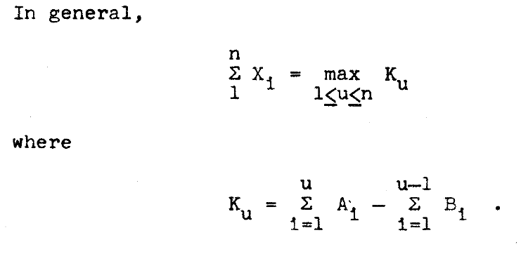
The proof starts by computing the exact formula for the sum of inactive periods of machine B (the sum of the \(X_i\) above). Different item orders will lead to different values for this sum, and we can show that an order is optimal if it follows the following rule:
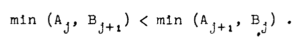
Item \(j\) precedes item \(j+1\) if In the original:
\[ \min\left(A_j, B_{j+1}\right) < \min\left(A_{j+1}, B_j\right). \]
It can be easily proved that this rule is transitive, therefore establishing a total order on the possible schedules, and implying the existence of a minimal schedule (unique up to items with identical durations).
A small implementation
Here is a minimal implementation of the algorithm as described above:
def johnsons_rule(items: list[tuple[int, int]]) -> list[int]:
    # Sort items by the duration for either machine
    sorted_indices = sorted(
        range(len(items)), key=lambda i: min(items[i])
    )
    front: list[int] = []  # Items placed at the front
    back: list[int] = []  # Items placed at the back
    for i in sorted_indices:
        tA, tB = items[i]
        if tA <= tB:
            front.append(i)
        else:
            back.append(i)
    back.reverse()
    return front + back
However in Python we can also sort the list of items using a comparison function. Using the comparison function from the proof above directly, we get:
import functools

def johnsons_rule_direct(items: list[tuple[int, int]]) -> list[int]:
    return sorted(
        range(len(items)),
        key=functools.cmp_to_key(
            lambda i, j: (
                min(items[i][0], items[j][1])
                - min(items[j][0], items[i][1])
            )
        ),
    )
We can now compute the schedule:
from dataclasses import dataclass
from collections.abc import Generator

@dataclass
class ItemSchedule:
    item_id: int
    machineA: tuple[int, int]
    machineB: tuple[int, int]


def compute_schedule(
    items: list[tuple[int, int]], order: list[int]
) -> Generator[ItemSchedule]:
    endA = 0
    endB = 0
    for i in order:
        tA, tB = items[i]
        startA = endA
        endA = startA + tA
        startB = max(endA, endB)
        endB = startB + tB
        yield ItemSchedule(
            item_id=i,
            machineA=(startA, endA),
            machineB=(startB, endB),
        )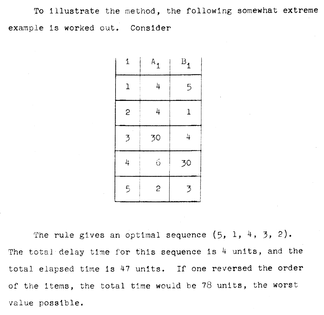
On the example from the paper, we get:
Optimal order: [4, 0, 3, 2, 1]
Sorted items: [(2, 3), (4, 5), (6, 30), (30, 4), (4, 1)]
Schedule:
  Item 4: machine A (0, 2), machine B (2, 5)
  Item 0: machine A (2, 6), machine B (6, 11)
  Item 3: machine A (6, 12), machine B (12, 42)
  Item 2: machine A (12, 42), machine B (42, 46)
  Item 1: machine A (42, 46), machine B (46, 47)
As a bonus, the implementation in BQN:
items←⟨4‿5,4‿1,30‿4,6‿30,2‿3⟩
# Naive version
JohnsonsRuleNaive←{((0⊸⊑𝕨)⌊1⊸⊑𝕩)<(0⊸⊑𝕩)⌊1⊸⊑𝕨}
# Array-oriented version
JohnsonsRule←{<´⌊´˘⍉𝕨≍⌽𝕩}
# Sort the items according to the rule
(⍒JohnsonsRule⌜˜)⊸⊏items
Which returns
⟨ ⟨ 2 3 ⟩ ⟨ 4 5 ⟩ ⟨ 6 30 ⟩ ⟨ 30 4 ⟩ ⟨ 4 1 ⟩ ⟩as expected.